The dance of bats and bells
When you study physics you are taught to build models to describe phenomena and to make future predictions based on what you cobble together. It is somehow implicit that if you can assemble some good models, you will get good results. In this scheme, which takes the name of determinism, everything is linked to a cause and the world appears as a necessary consequence of what was. Although this vision may look suggestive, this is way far from being real.
Many deterministic systems are so highly dependent on the initial conditions that small perturbations of them affect deeply the evolution of the systems, making any prediction untrustworthy. In addition to this, in many contexts it is not possible to know the initial conditions with arbitrary precision. The system will appear to evolve in a chaotic manner: this is the deterministic chaos.
A Toy Model
One of the most fascinating chaotic systems is the chaotic magnetic pendulum.
Let's suppose to have three magnets on a plane and a pendulum oscillating over them. The length of the pendulum is assumed to be long enough to approximate the portion of the sphere where the pendulum moves with a flat surface. The latter is kept fixed at a distance $D$ from the magnets, which attract the pendulum and affect its motion. The recipe we follow to build a simple but satisfying model is the following:
- gravity: the further the pendulum is from its rest position, the stronger the gravity force pushes the pendulum back to the origin;
- friction: faster the pendulum moves, the larger the friction with the air;
- magnetic attraction: the further the pendulum is from a magnet, the weaker the attraction.
Setting the origin of a reference system at the resting point of the pendulum in the absence of the magnets, the deterministic equations describing this motion are the following:
$\frac{d^{2}x}{d^{2}t} = -R\frac{dx}{dt} - Gx - m\sum_{i=1} \frac{x-x_i}{((x-x_i)^2+(y-y_i)^2+D^2))^\frac{3}{2}}$
$\frac{d^{2}y}{d^{2}t} = -R\frac{dy}{dt} - Gy - m\sum_{i=1} \frac{y-y_i}{((x-x_i)^2+(y-y_i)^2+D^2))^\frac{3}{2}}$
where ($x_i$,$y_i$) are the coordinates of the i-th magnet, $R$ the coefficient that couples the velocity of the pendulum with the frictional force, $G$ the gravity interaction and $m$ the strength of the magnets. Notice that setting $m=0$ leads to the standard equations of a damped pendulum.
Solving the equations
The only way to probe the motion of this system is to compute the solutions numerically. Although for many projects Python and its libraries are efficient tools, this is an example where the reduced running time of C is a trump card to play. That's why I opted to build a C library and import the compiled file into a Jupyter Notebook which is used to plot the result. I used the Euler-Cromer algorithm to integrate the equations, but no more chatting and let's dive into the code!
First, we need to import the libraries we are going to use and declare the constants we will use in the script. Of course, it is not mandatory to define the constants, but I think it is a good practice to keep everything tidy. Moreover, the constants defined in this way - they take the name of macros - have the largest scope possible: their values are accessible by any function.
#include <stdio.h>
#include <math.h>
#include <time.h>

#define L 10 /*reciprocal distance magnets*/
#define D2 0.2
#define dt 0.05
#define gravity .2
#define friction .2
#define magnetic_coupling 13
#define MAX_STEP 28000
#define rad2grad 57.2958
On this occasion, it is equally convenient to define a struct, a sort of container grouping several related variables into one place.
struct point {

    double x;
    double y;
    double v_x;
    double v_y;
    double a_x;
    double a_y;
 };
struct point magnets[3];

struct point init_point(double ,double ,double ,double );
void  init_magnets();
double basin(double,double,double,double);
void trajectory(double,double,double,double,char *);
struct point eulero_cromer(struct point);
int stop_integration(struct point);
double my_atan(double , double );
In the code above the struct point is a group of variables describing the dynamic state of an object in terms of position, velocity and acceleration. We also define magnets an array of struct point, one for each of the three magnets.
Always in the spirit of building a clean code, I wrote two functions to initialize the state of the pendulum and the positions of the magnets. The function init_point() takes as arguments the four initial conditions for the pendulum and returns the corresponding point representation. Notice that the components of the acceleration are computed by combining the three terms discussed above: gravity, magnetic coupling and friction.
To do that, it is necessary to fix the positions of the magnets. This task is done by the function init_magnets(), which fixes the 3 magnets in a way to form an equilateral triangle of sides L centred on the origin.
struct point init_point(double x_0,double y_0,double v_x_0,double v_y_0){

    struct point P;
    double r,f_x,f_y;
    P.x = x_0;
    P.y = y_0;
    P.v_x = v_x_0;
    P.v_y = v_y_0;


    for(int i=0;i<3;i++){
        r = pow(pow((P.x-magnets[i].x),2)+pow((P.y-magnets[i].y),2) + D2,1.5);
        f_x = f_x + magnetic_coupling*(magnets[i].x-P.x)/r;
        f_y = f_y + magnetic_coupling*(magnets[i].y-P.y)/r;
    }

    P.a_x = - gravity*P.x - friction*P.v_x + f_x;
    P.a_y = - gravity*P.y - friction*P.v_y + f_y;
    return P;
}

void init_magnets(){


    magnets[0].x = -L/2;
    magnets[0].y = -L/2*tan(M_PI/6);

    magnets[1].x = 0;
    magnets[1].y = L*(cos(M_PI/6)-0.5*tan(M_PI/6));

    magnets[2].x = L/2;
    magnets[2].y = -L/2*tan(M_PI/6);
    return;
}
Now that the initial conditions are set, everything is ready to explore the dynamic of the system. We aim to plot the trajectory of the pendulum given a set of initial conditions and draw the so-called basins of attractions. Because of the presence of friction, we know that the pendulum sooner or later will stop somewhere. Even without making any complex computation, we expect there will be 4 possible resting points: three in correspondence with the magnets and one in ($0$,$0$). The set of initial conditions sharing the same resting point forms the so-called basin of attraction of the resting point, the attractor.
The functions I prepared are the following:
void trajectory(
    double x_0,
    double y_0,
    double v_x_0,
    double v_y_0,
    char * filename){

    double r,v,theta;
    int count;
    struct point P;
    FILE *fp = fopen(filename,"w");

    init_magnets();
    P = init_point(x_0,y_0,v_x_0,v_y_0);
    count = 0;
    while(count<MAX_STEP){
        count ++;
        v = sqrt(pow(P.v_x,2) + pow(P.v_y,2));
        r = sqrt(pow(P.x,2)+pow(P.y,2));
        theta = myAtan(P.x,P.y);
        fprintf(fp,"%f,%f,%f,%f,%f,%f,%f\n",P.x,P.y,r,theta,P.v_x,P.v_y,v);
        P = eulero_cromer(P);
        if(stop_integration(P)){
            break;
        }
    }
    return;
}

double basin(double x_0,
            double y_0,
            double v_x_0,
            double v_y_0){

    double r,v,theta;
    int count;
    struct point P;
    init_magnets();
    P = init_point(x_0,y_0,v_x_0,v_y_0);
    count = 0;
    while(count<MAX_STEP){
        count ++;
        P = eulero_cromer(P);
        if(stop_integration(P)){
            break;
        }
    }
    return my_atan(P.x,P.y);
 }
Of course, if one knows the complete trajectory of the pendulum starting its motion from the point $P=(x_0,y_0,v_{x_{0}},v_{y_{0}})$ then it's known where the pendulum is resting too, and so which is the attractor of $P$. However, I decided to code two different functions to avoid saving each point of the trajectory when probing the basins of attractions. Indeed drawing the basins of attraction is an expensive task, since what we need to do is to solve the equations of the motion for all the possible initial conditions.
Last but not least, here are the functions euler_cromer(), stop_integration() and my_atan() which are essential to update the state of the pendulum, check if it is still moving or not and compute the angle between the x-axis and the vector that joins the origin with any point of the plane.
struct point euler_cromer(struct point state){

    struct point next_state;
    double x_next,y_next,vx_next,vy_next;
    double f_x = 0;
    double f_y = 0;
    double r_xi = 0;

    vx_next = state.v_x + state.a_x*dt;
    vy_next = state.v_y + state.a_y*dt;
    x_next = state.x + vx_next*dt;
    y_next = state.y + vy_next*dt;

    next_state.x = x_next;
    next_state.y = y_next;
    next_state.v_x = vx_next;
    next_state.v_y = vy_next;

    for(int i=0;i<3;i++){
        r_xi = pow(pow((next_state.x-magnets[i].x),2)+pow((next_state.y-magnets[i].y),2) + D2,1.5);
        f_x = f_x + magnetic_coupling*(magnets[i].x-next_state.x)/r_xi;
        f_y = f_y + magnetic_coupling*(magnets[i].y-next_state.y)/r_xi;
    }
    next_state.a_x=- gravity*next_state.x - friction*next_state.v_x + f_x;
    next_state.a_y=- gravity*next_state.y - friction*next_state.v_y + f_y;

    return next_state;

}

int stop_integration(struct point state){

    double norm2_v,norm2_a;
    norm2_v = pow(state.v_x,2)+pow(state.v_y,2);
    norm2_a = pow(state.a_x,2)+pow(state.a_y,2);
    if(norm2_v<0.001 && norm2_a<0.001){
        return 1;
    }
    return 0;
}

double myAtan(double x,double y){

    if((pow(x,2)+pow(y,2))<THRESHOLD_R){
        return 0;
    }

    if(x<0 && y>0){
        return 180+atan(y/x)*rad2grad;
    }
    if(x<0 && y<0){
        return 180+atan(y/x)*rad2grad;
    }
    return atan(y/x)*rad2grad;
}
Running the code
The code is ready and we can finally run the main functions trajectory() and basins() to plot and study the main results. I have found really useful this article which explains how to wrap a C library in Python.
The snippet below is a simple example of how to wrap everything with ctypes and use the function trajectory()to compute numerically the trajectory of the pendulum with initial conditions $(x_0=8,y_0=1,v_{x_{0}}=-4,v_{y_{0}}=6)$ and save the results in traj1.csv.
import numpy as np
from math import tan,sin,cos,sqrt
from cmath import pi
from numpy.linalg import norm
import pandas as pd
import matplotlib.pyplot as plt
from numpy.ctypeslib import ndpointer
import ctypes
lib = ctypes.CDLL('./chaos.so') #import the pre-compiled C library
import os
import time
import plotly.express as px
import imageio


basin = lib.basin #importing the function basin
basin.restype = ctypes.c_double
basin.argtypes = [ctypes.c_double,
                     ctypes.c_double,
                     ctypes.c_double,
                     ctypes.c_double,
                     ]

trajectory = lib.trajectory #importing the function basin
trajectory.argtypes = [ctypes.c_double,
                     ctypes.c_double,
                     ctypes.c_double,
                     ctypes.c_double,
                     ctypes.c_char_p
                    ]

trajectory(8,1,-4,6,'traj1.csv'.encode('utf-8'))
Moreover, one can compute the potential $V(x,y)$ for all the points of the plane and visualize the motion of the pendulum with a GIF. The function $V(x,y)$ is defined as:
$f_x=\frac{d^2x}{d^2t}=-\frac{dV}{dx}$
$f_y=\frac{d^2y}{d^2t}=-\frac{dV}{dy}$
where $f_x$ and $f_y$ are the components of the force acting on a pendulum of unitary mass. These equations tell us that we need to integrate the equation of the motion to get the potential and that the pendulum is driven from points of high potential towards points of lower potential. Colouring the space according to the values of $V$ helps to visualize which are the system's attractors, and so predict what will happen to the pendulum when moving around the plane. In other words, we can map the pendulum to a ball rolling on a conical plane - gravity pushes the pendulum to the point $(0,0)$ - having three wells in correspondence of the three magnets.
Finally, let's see what we get if we study the basins of attractions. As we mentioned before, the system shows four points of attraction: the three magnets and the origin (0,0). We can first imagine assigning a colour to each of these points and letting the system evolve from the initial condition $(x,y,v_{x_{0}}=0,v_{x_{0}}=0)$ and colour the point $(x,y)$ by using the colour of the attractor that catches the pendulum. Probing the plane on different scales we obtain these beautiful pictures: an infinite dance of bats and bells.
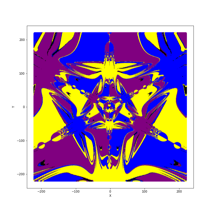
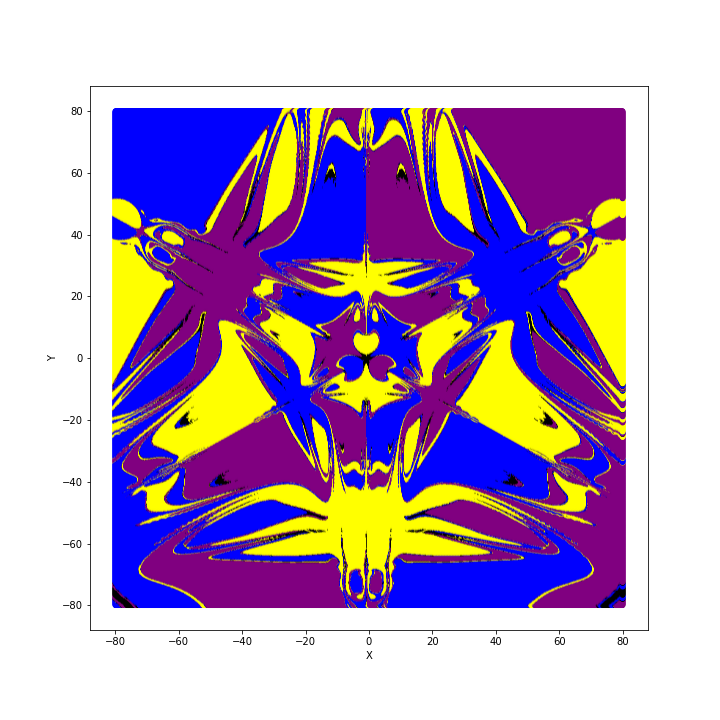
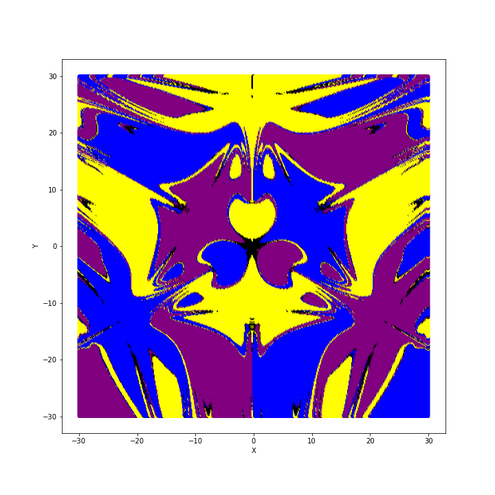
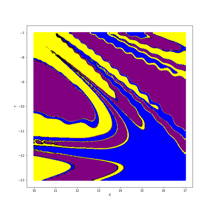
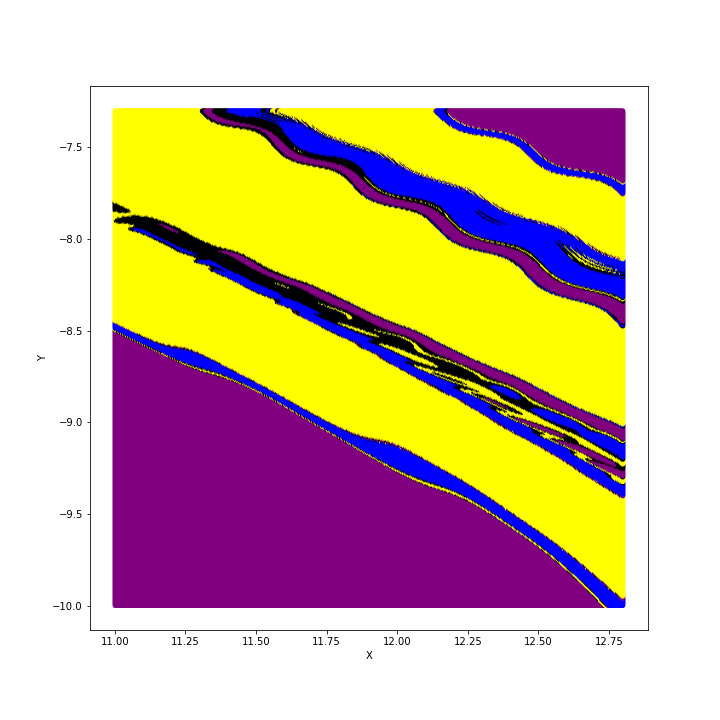
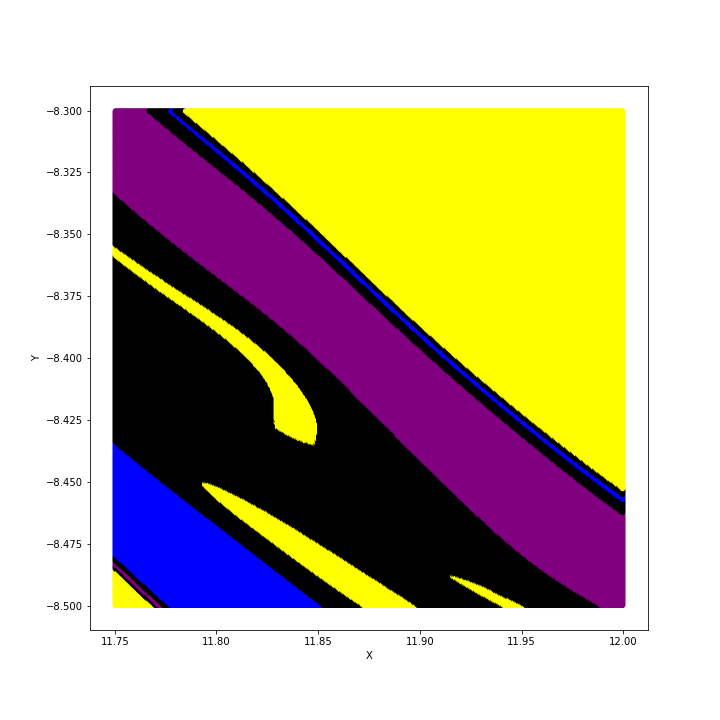
The first thing that we notice is that these pictures show a high degree of symmetry. This is not surprising since the magnets are identical and they are placed forming an equilateral triangle. The second thing is that the first two pictures look truly similar, although the first one covers a wider area. This property of scale-invariance is the same that characterizes a large class of objects called fractals. Common examples of fractals in nature are snowflakes, trees branching and lightning. Moreover, if we inspect the boundaries of the basins of attraction it is not rare to come across sub-boundaries. The last three pictures are progressive zooms which show finer and finer details. In the very last picture, we see a series of thin black, blue and black again bars between the purple and yellow domains. Such fragmented basins of attraction are clear manifestations of the chaos: releasing the pendulum from a slightly different point leads to a completely different evolution. If you want to know more about which quantitative analysis can be done to characterize the unpredictability associated with the basins of attraction, you can have a look at this paper by Alvar Daza and his colleagues.
Final thoughts
In this short article, we have seen a chaotic behaviour emerging from a relatively simple system. We wrote a couple of differential equations using a standard recipe, we solved them and we got such rich and unexpected results. What if had studied a more complex system? What if we had tried to model the traffic of a big city or the activities of the human brain? In this interesting paper Deterministic nonlinear chaos in brain function and borderline psychopathological phenomena a nonlinear and chaotic mechanism is pointed out as what guarantees a sane functionality of the brain, suggesting that after all chaos and order are possibly two sides of the same coin: the beauty of Nature.