Islands, Peninsulas and Ponds

Weeks ago, I came across the video on Medium titled Google Coding Interview With Ben Awad. Although I didn't watch it completely, I found the coding challenge presented in the video to be very interesting. Moreover, I had the impression that this challenge was, in some way, a variation of a mathematical problem I encountered during my studies – percolation in a 2D square lattice.

The Challenge

What the candidate is asked to implement is the following:

"Given a 2-dimensional matrix populated only by 1s and 0s, the algorithm must detect all the islands within the matrix. An island is simply an aggregation of 1s that is surrounded by 0s, and none of the elements of the islands must have any contact with the four sides of the matrix. Contact are only possible through the nearest neighbors."

In other picturesque words, we can envision the matrix as a 2-dimensional discrete world where each elementary site can represent either a piece of land (if the cell element is 1) or a pond (if the cell element is 0). Our task is to identify the regions that are inaccessible without the use of a boat from the boundary of this two-dimensional world.

A solution

If we can design an algorithm that, given a site, returns all the sites connected to it, then we would easily solve the challenge. In fact, you can easily imagine identifying the connected sites for each of the sites placed within the boundaries of the matrix. Connected sites form what is usually called a cluster, and to maintain the analogy with ponds and islands, we can say that a cluster attached to at least one side of the matrix can be seen as a peninsula.

It is also evident that if we can distinguish all the peninsulas, what will remain are the islands—the clusters not attached to any boundary—and the water of course.

Implementing such a function in Python is not too difficult. I chose to start by building the  node class. A node object is used to represent the elementary sites that form clusters. Each node has a parent (except for the root node), and we can uniquely identify it by its coordinates ( x, y). Additionally, a site can have children, which are the nodes attached to it. The structure that is created is a particular type of graph called a tree. The root site can have no more than 4 children, while all the others can have between 0 and 3 children. If a node has 0 children, it is a leaf in the tree.

Of course, there are no privileged sites and so the choice of the root note is completely arbitrary. We only need a starting point from which to expand the cluster.

To initialize a node object, the class requires specifying the parent of the node (which can be set to None if we are creating the root node), its position (x, y), and the root of the tree to which it is attached. Additionally, two methods were added to perform basic operations. The is_leaf method simply checks if a node is a leaf by computing the number of nodes listed as children, and the append_children method, which takes another node as input and appends it to the list of children.

class node:

    def __init__(self,parent,x,y,root):

        self.parent = parent
        self.x = x
        self.y = y
        self.root = root
        self.children = []
    
    def is_leaf(self):
        
        if(len(self.children)==0):
            return True
        else:
            return False
    
    def append_children(self,B):

        self.children.append(B)
        return 

This class, by itself, can't find any clusters. It is simply a way to model the elementary objects that compose the clusters and to prepare a structure to organize the information.

What really takes on the dirty job is the function extend_tree. As the name suggests, the goal of this function is to construct a tree of nodes connected to a given root node. This function takes the matrix where the sites exist and the color we wish to assign to the detected cluster. The color of the cluster serves as a label, as we expect that when given two random sites, there is a probability that they belong to two different clusters. We will delve deeper into this aspect later; for now, it's important to understand that our objective is to label clusters, and a convenient way to do that is by using colors represented as integer numbers.

If you examine the few lines below, you will notice that:

1. the initial step involves constructing a list called stack, which initially contains only one element, the root node. Additionally, we save the size of the square matrix, denoted as N.
2. as long as the stack list is not empty, we extract the most recent node from the stack, which is assigned to the variable current_node. Then, we color the cell of the matrix where the node seats.
3. after extracting the current node, we proceed to inspect its neighborhood using a for loop. One by one, if the neighboring cells are part of the land (i.e., connected sites), we elevate them to a corresponding node object. This node object is then appended to the list of children of the current node and also added to the stack list for further exploration.

Coloring the already visited nodes with a color (integer) is crucial to ensure the algorithm's termination. By setting color=2, for example, the function will mark all the matrix elements connected to the root node with the value 2. Subsequently, the if clause within the for loop will prevent the algorithm from stepping outside the boundaries of the matrix and revisiting nodes that have already been visited.

This mechanism ensures that the algorithm can properly explore the cluster without getting stuck in infinite loops or redundant visits to the same nodes.

Finally, we wrap everything together and check out the peninsulas that are attached to at least one of the four sides of the square matrix.

#matrix generation
N = 1500
p = 0.58
matrix = np.random.choice([0, 1], size=(N, N), p=[1-p, p])
colored_matrix=matrix.copy()

color = 1
roots_list = []

#exploring up and buttom sides
for y in range(matrix.shape[0]):
    for x in [0,N-1]:
        if(colored_matrix[x][y]==1):
            color +=1 #change the color for the new cluster
            root = node(parent=None,root=None,x=x,y=y)
            root.root = root
            roots_list.append(root) #save roots into a list
            extend_tree(root,matrix=colored_matrix,color=color)


#exploring left and right sides
for x in range(matrix.shape[0]):
    for y in [0,N-1]:
        if(colored_matrix[x][y]==1):
            color +=1 #change color for the new cluster
            root = node(parent=None,root=None,x=x,y=y)
            root.root = root
            roots_list.append(root) #save roots into a list
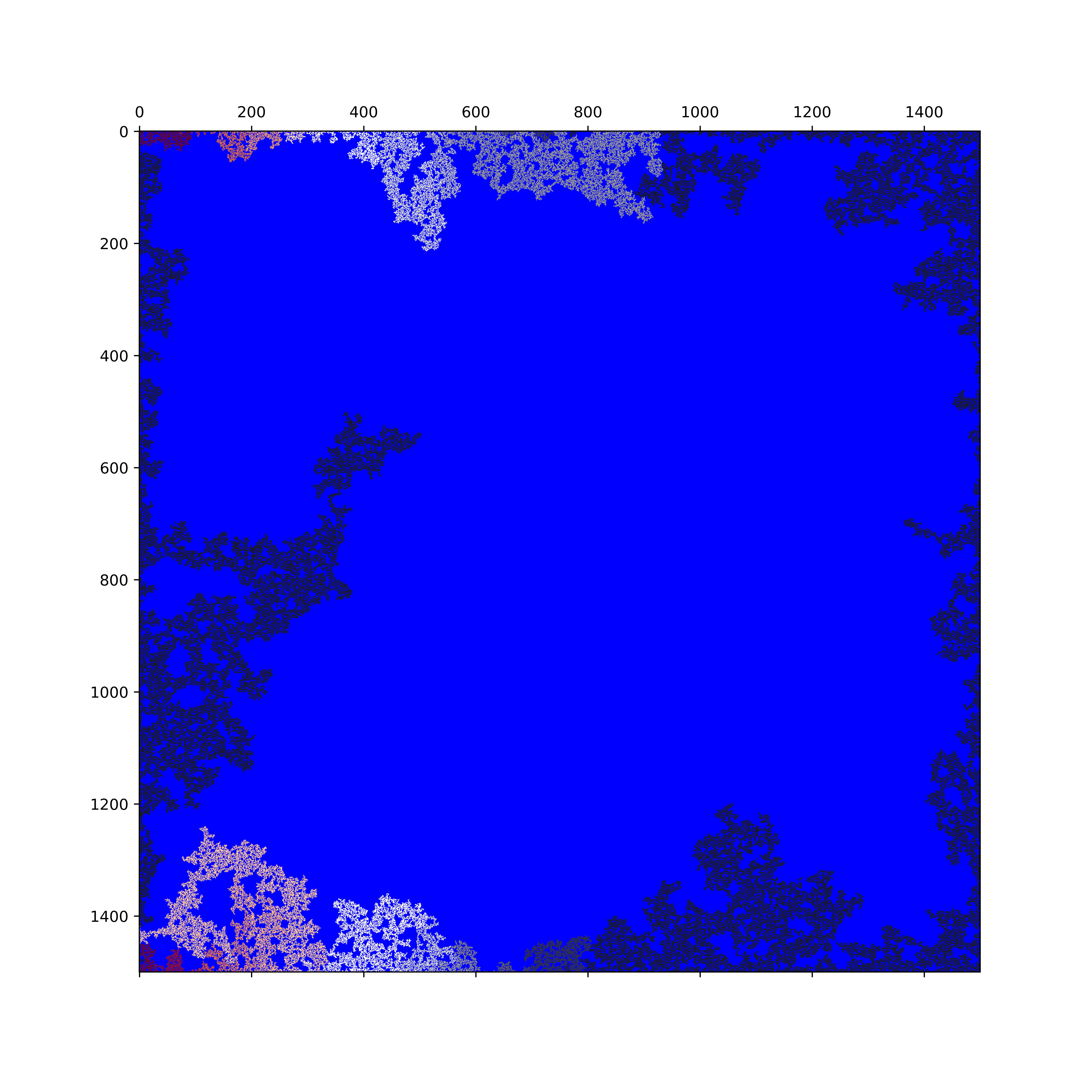
            extend_tree(root,matrix=colored_matrix,color=color)

Since we label all the sites that are visited by a color different from 1, it is possible to easily filter out the 1s, which correspond to inner sites that are not connected to any of the sides of the matrix, and plot the peninsulas that are found. Because of the stochastic nature of the process, it is not expected to see peninsulas of the same size.

Moreover, as we save all the root nodes in the list roots_list, it is possible to walk through all the clusters by extracting the coordinates of the descendants. To achieve this, I created the function extract_coordinates:

def extract_coordinates(root):

    list_coordinates = []
    stack = [root]

    while stack:
        node = stack.pop()
        list_coordinates.append((node.x,node.y))

        for child in node.children:
            stack.append(child)
    
    return list_coordinates

And with a simple for loop it is possible to identify the largest cluster and its size:

clusters_corrds = [extract_coordinates(r) for r in roots_list]
max_cluster = max(clusters_corrds, key=lambda x: len(x))
print(f"Largest cluster size: {len(max_cluster)} sites")

Criticality

In coding challenges, candidates are typically provided with inputs. In this case, the input to be processed is a matrix populated with 1s and 0s. Naturally, I had to generate one to test the algorithm I created. As shown in the snippet above, I set the probability $p$ to determine whether a cell in the matrix contains a 1.

It is realistic to expect that for small values of $p$, we will not observe very large clusters. Conversely, as $p$ approaches 1, we anticipate a massive cluster spanning from one side to the other almost filling the whole space. Additionally, it is reasonable to assume the existence of a critical value of $p$, denoted as $p_c$, which serves as the watershed between a regime with only finite clusters ($p < p_c$) and a regime with an infinite spanning cluster ($p \geq p_c$), which is the manifestation of percolation. In other words, the system is expected to undergo what is known as a phase transition, where the expected number of 1 sites (lands) belonging to the infinite cluster (mainland) serves as the order parameter. In the case of a 2-dimensional square lattice, $p_{c}=0.5927$.

It is worth clarifying that we will never detect an infinite spanning cluster as when using a computer we are always limited by the memory of the machine. However, we can imagine working with an infinite matrix, i.e., $N \rightarrow \infty$. In this regime, the tools developed by scaling theories give many interesting results, the main interesting being:

1. if we define the correlation length $\xi$ as the average squared distance between two cluster sites belonging to the same finite cluster, it diverges at the criticality: $ \xi \propto |p-p_{c}|^{-\nu}$

2. a diverging correlation length allows the emergence of fractals structure.

Intuitively, close to criticality, the biggest finite clusters merge into a unique entity whose scale is given by the correlation length, which explodes. The structure is said to be self-similar for scales smaller than the correlation length. As we get closer to $p_{c}$, the correlation length diverges, and a massive fractal object emerges. In this case, the structure looks the same at all scales.

Another way to put it, if one computes the average number of clusters of size s per lattice site at the critical point $n_{p_{c}}(s)$ , one finds a power law decay:

$$ n_{p_{c}}(s) \propto s^{-\tau}$$

Power laws are the essence of scale invariance and self-similarity; in fact, if $f(z)$ is a power law, it is true that $\frac{f(ay)}{f(ax)} = \frac{f(y)}{f(x)}$.

In the case of the average number of clusters, we can conclude that if we zoom in on the system with a lens, i.e., we reduce the scale of the system, we would see the same invariant picture. You can interact with the plot below, which displays the system in proximity to the criticality. Try exploring the fractal structure by observing the holes left by the biggest clusters, which are populated by smaller clusters.

Further readings

Of course, this post is not meant to be an exhaustive note on Percolation Theory, which is probably one of the most fascinating topics I encountered during my lectures on Statistical Field Theory while pursuing my Master's degree in Phisics of Complex Systems. If you are interested in delving deeper into the subject, I highly recommend Introduction to Percolation Theory by Dietrich Stauffer and Amnon Aharon. Additionally, a valuable and more affordable source is the lecture note Percolation Theory by Dr Kim Christensen.